How We Built a Vectorized Execution Engine
CockroachDB is an OLTP database, specialized for serving high-throughput queries that read or write a small number of rows. As we gained more usage, we found that customers weren’t getting the performance they expected from analytic queries that read a lot of rows, like large scans, joins, or aggregations. In April 2018, we started to seriously investigate how to improve the performance of these types of queries in CockroachDB, and began working on a new SQL execution engine. In this blog post, we use example code to discuss how we built the new engine and why it results in up to a 4x speed improvement on an industry-standard benchmark.
OLTP databases, including CockroachDB, store data in contiguous rows on disk and process queries a row of data at a time. This pattern is optimal for serving small queries with high throughput and low latency, since the data in the rows are stored contiguously, making it more efficient to access multiple columns from the same row. Modern OLAP databases, on the other hand, typically are better at serving large queries, and tend to store data in contiguous columns and operate on these columns using a concept called vectorized execution. Using vectorized processing in an execution engine makes more efficient use of modern CPUs by changing the data orientation (from rows to columns) to get more out of the CPU cache and deep instruction pipelines by operating on batches of data at a time.
In our research into vectorized execution, we came across MonetDB/X100: Hyper-Pipelining Query Execution, a paper that outlines the performance deficiencies of the row-at-a-time Volcano execution model that CockroachDB’s original execution engine was built on. When executing queries on a large number of rows, the row-oriented execution engine pays a high cost in interpretation and evaluation overhead per tuple and doesn’t take full advantage of the efficiencies of modern CPUs. Given the key-value storage architecture of CockroachDB, we knew we couldn’t store data in columnar format, but we wondered if converting rows to batches of columnar data after reading them from disk, and then feeding those batches into a vectorized execution engine, would improve performance enough to justify building and maintaining a new execution engine.
To quantify the performance improvements, and to test the ideas laid out in the paper, we built a vectorized execution engine prototype, which yielded some impressive results. In this tutorial-style blog post, we take a closer look at what these performance improvements look like in practice. We also demonstrate why and how we use code generation to ease the maintenance burden of the vectorized execution engine. We take an example query, analyze its performance in a toy, row-at-a-time execution engine, and then explore and implement improvements inspired by the ideas proposed in the MonetDB/x100 paper. The code referenced in this post resides in https://github.com/asubiotto/vecdeepdive, so feel free to look at, modify, and/or run the code and benchmarks while you follow along.
What’s in a SQL operator?
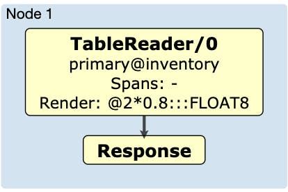
To provide some context, let’s look at how CockroachDB executes a simple query, SELECT price * 0.8 FROM inventory, issued by a fictional retail customer that wants to compute a discounted price for each item in her inventory. Regardless of which execution engine is used, this query is parsed, converted into an abstract syntax tree (AST), optimized, and then executed. The execution, whether distributed amongst all nodes in a cluster, or executed locally, can be thought of as a chain of data manipulations that each have a specific role, which we call operators. In this example query, the execution flow would look like this:
!executionflow
You can generate a diagram of the physical plan by executing EXPLAIN (DISTSQL)on the query. As you can see, the execution flow for this query is relatively simple. The TableReader operator reads rows from the inventory table and then executes a post-processing render expression, in this case the multiplication by a constant float. Let’s focus on the render expression, since it’s the part of the flow that is doing the most work.
Here’s the code that executes this render expression in the original, row-oriented execution engine used in CockroachDB (some code is omitted here for simplicity):
func (expr *BinaryExpr) Eval(ctx *EvalContext) (Datum, error) {
	left, err := expr.Left.(TypedExpr).Eval(ctx)
	if err != nil {
		return nil, err
	}
	right, err := expr.Right.(TypedExpr).Eval(ctx)
	if err != nil {
		return nil, err
	}
	return expr.fn.Fn(ctx, left, right)
}
The left and right side of the binary expression (BinaryExpr) are both values wrapped in a Datum interface. The BinaryExpr calls expr.fn.Fn with both of these as arguments. In our example, the inventory table has a FLOAT price column, so the Fnis:
Fn: func(_ *EvalContext, left Datum, right Datum) (Datum, error) {
        return NewDFloat(*left.(*DFloat) * *right.(*DFloat)), nil
}
In order to perform the multiplication, the Datum values need to be converted to the expected type. If, instead, we created a price column of type DECIMAL, we would cast 0.8 to a DECIMAL and then construct a BinaryExpr with a different Fn specialized for multiplying DECIMALs.
We now have specialized code for multiplying each type, but the TableReader doesn’t need to worry about it. Before executing the query, the database creates a query plan that specifies the correct Fn for the type that we are working with. This simplifies the code, since we only need to write specialized code as an implementation of an interface. It also makes the code less efficient, as each time we multiply two values together, we need to dynamically resolve which Fn to call, cast the interface values to concrete type values that we can work with, and then convert the result back to an interface value.
Benchmarking a simple operator
How expensive is this casting, really? To find the answer to this question, let’s take a similar but simpler toy example:
type Datum interface{}

// Int implements the Datum interface.
type Int struct {
    int64
}

func mulIntDatums(a Datum, b Datum) Datum {
	aInt := a.(Int).int64
	bInt := b.(Int).int64
	return Int{int64: aInt * bInt}
}

// ...

func (m mulOperator) next() []Datum {
	row := m.input.next()
	if row == nil {
		return nil
	}
	for _, c := range m.columnsToMultiply {
		row[c] = m.fn(row[c], m.arg)
	}
	return row
}
This is a type-agnostic single operator that can handle multiplication of an arbitrary number of columns by a constant argument. Think of the input as returning the rows from the table. To add support for DECIMALs, we can simply add another function that multiplies DECIMALs with a mulFn signature.
We can measure the performance of this code by writing a benchmark (see it in our repo). This will give us an idea of how fast we can multiply a large number of Int rows by a constant argument. The benchstat tool tells us that it takes around 760 microseconds to do this:
$ go test -bench “BenchmarkRowBasedInterface$” -count 10 > tmp && benchstat tmp && rm tmp
name               	time/op
RowBasedInterface-12	760µs ±15%
Because we have nothing to compare the performance against at this point, we don’t know if this is slow or not.
We’ll use a “speed of light” benchmark to get a better relative sense of this program’s speed. A “speed of light” benchmark measures the performance of the minimum necessary work to perform an operation. In this case, what we really are doing is multiplying 65,536 int64s by
- The result of running this benchmark is:
$ go test -bench "SpeedOfLight" -count 10 > tmp && benchstat tmp && rm tmp
name               	time/op
SpeedOfLight-12    	19.0µs ± 6%
This simple implementation is about 40x faster than our earlier operator!
To try to figure out what’s going on, let’s run a CPU profile on BenchmarkRowBasedInterface and focus on the mulOperator. We can use the -o option to obtain an executable, which will let us disassemble the function with the disasm command in pprof. As we will see below, this command will give us the assembly that our Go source code compiles into, along with approximate CPU times for each instruction. First, let’s use the top and list commands to find the slow parts of the code.
$ go test -bench "BenchmarkRowBasedInterface$" -cpuprofile cpu.out -o row_based_interface
…
$ go tool pprof ./row_based_interface cpu.out
(pprof) focus=mulOperator
(pprof) top
Active filters:
   focus=mulOperator
Showing nodes accounting for 1.99s, 88.05% of 2.26s total
Dropped 15 nodes (cum **D**on’t **R**epeat **Y**ourself). The situation seems even worse if we consider that in a real database engine, there would be far more than two types to support. If someone were to slightly change the multiplication functionality (for example, adding overflow handling), they would have to rewrite every single operator, which is tedious and error-prone. The more types, the more work one has to do to update code.

## Generating code with templates

Thankfully, there is a tool we can use to reduce this burden and keep the good performance characteristics of working with concrete types. The [Go templating engine](https://golang.org/pkg/text/template/) allows us to write a code template that, with a bit of work, we can trick our editor into treating as a regular Go file. We have to use the templating engine because the version of Go we are currently using does not have support for generic types. Templating the multiplication operators would look like this (full template code is in [row_based_typed_tmpl.go](https://github.com/asubiotto/vecdeepdive/blob/90db3ceba8a048743d23991b4db234f070dcec57/row_based_typed_tmpl.go)):

**`// {{/*
type _GOTYPE interface{}

// _MULFN assigns the result of the multiplication of the first and second
// operand to the first operand.
func _MULFN(_ TypedDatum, _ interface{}) {
	panic("do not call from non-templated code")
}
// */}}
// {{ range .}}
type mul_TYPEOperator struct {
	input             TypedOperator
	arg               _GOTYPE
	columnsToMultiply []int
}
func (m mul_TYPEOperator) next() []TypedDatum {
	row := m.input.next()
	if row == nil {
		return nil
	}
	for _, c := range m.columnsToMultiply {
		_MULFN(row[c], m.arg)
	}
	return row
}
// {{ end }}`**

The accompanying code to generate the full `row_based_typed.gen.go` file is located in [`row_based_type_gen.go`](https://github.com/asubiotto/vecdeepdive/blob/90db3ceba8a048743d23991b4db234f070dcec57/row_based_typed_gen.go)). This code is executed by running `go run .` to run the `main()` function in `generate.go` (omitted here for conciseness). The generator will iterate over a slice and fill the template in with specific information for each type. Note that there is a prior step that is necessary in order to consider the `row_based_typed_tmpl.go` file valid Go. In the template, we use tokens that are valid Go (e.g. _GOTYPE and _MULFN). These tokens’ declarations are wrapped in template comments and removed in the final generated file.

For example, the multiplication function (`_MULFN`) is converted to a method call with the same arguments:

**`// Replace all functions.
mulFnRe := regexp.MustCompile(`_MULFN\((.*),(.*)\)`)
s = mulFnRe.ReplaceAllString(s, `{{ .MulFn "$1" "$2" }}`)`**

`MulFn` is called when executing the template, and then returns the Go code to perform the multiplication according to type-specific information. Take a look at the final generated code in [row_based_typed.gen.go.](https://github.com/asubiotto/vecdeepdive/blob/90db3ceba8a048743d23991b4db234f070dcec57/row_based_typed.gen.go))

The templating approach we took has some rough edges, and certainly is not a very flexible implementation. Nonetheless, it is a critical part of the real vectorized execution engine that we built in CockroachDB, and it was simple enough to build without getting sidetracked by creating a robust domain-specific language. Now, if we want to add functionality or fix a bug, we can modify the template once and regenerate the code for changes to all operators. Now that the code is a little more manageable and extensible, let’s try to improve the performance further.

NOTE: To make the code in the rest of this blog post easier to read, we won’t use code generation for the following operator rewrites.

## Batching expensive calls

Repeating our benchmarking process from before shows us some useful next steps.

**`$ go test -bench "BenchmarkRowBasedTyped$" -cpuprofile cpu.out -o row_typed_bench
$ go tool pprof ./row_typed_bench cpu.out

(pprof) list next
ROUTINE ======================== _~/scratch/vecdeepdive.mulInt64Operator.next in ~/scratch/vecdeepdive/row_based_typed.gen.go
 	1.26s  	1.92s (flat, cum) 85.71% of Total
     	.      	.  	8:    input         	TypedOperator
     	.      	.  	9:    arg           	int64
     	.      	. 	10:    columnsToMultiply []int
     	.      	. 	11:}
     	.      	. 	12:
 	180ms  	180ms 	13:func (m mulInt64Operator) next() []TypedDatum {
 	170ms  	830ms 	14:    row := m.input.next()
     	.      	. 	15:    if row == nil {
     	.      	. 	16:   	 return nil
     	.      	. 	17:    }
 	330ms  	330ms 	18:    for _, c := range m.columnsToMultiply {
 	500ms  	500ms 	19:   	 row[c].int64*= m.arg
     	.      	. 	20:    }
  	80ms   	80ms 	21:    return row
     	.      	. 	22:}`**

This part of the profile shows that approximately half of the time spent in the `mulInt64Operator.next` function is spent calling `m.input.next()` (see line 13 above). This isn’t surprising if we look at our implementation of `(*typedTableReader).next()`; it’s a lot of code just for advancing to the next element in a slice. We can’t optimize too much about the `typedTableReader`, since we need to preserve the ability for it to be chained to any other SQL operator that we may implement. But there is another important optimization that we can do: instead of calling the next function once for each row, we can get back a batch of rows and operate on all of them at once, without changing too much about `(*typedTableReader).next`. We can’t just get all the rows at once, because some queries might result in a huge dataset that won’t fit in memory, but we can pick a reasonably large batch size.

With this optimization, we have operators like the ones below. Once again, the full code for this new version is omitted, since there’s a lot of boilerplate changes. Full code examples can be found in [row_based_typed_batch.go](https://github.com/asubiotto/vecdeepdive/blob/master/row_based_typed_batch.go).

**`type mulInt64BatchOperator struct {
    input         	TypedBatchOperator
    arg           	int64
    columnsToMultiply []int
}

func (m mulInt64BatchOperator) next() [][]TypedDatum {
    rows := m.input.next()
    if rows == nil {
   	 return nil
    }
    for _, row := range rows {
   	 for _, c := range m.columnsToMultiply {
   		 row[c] = TypedDatum{t: Int64Type, int64: row[c].int64 * m.arg}
   	 }
    }
    return rows
}

type typedBatchTableReader struct {
    curIdx int
    rows   [][]TypedDatum
}

func (t *typedBatchTableReader) next() [][]TypedDatum {
    if t.curIdx >= len(t.rows) {
   	 return nil
    }
    endIdx := t.curIdx + batchSize
    if endIdx > len(t.rows) {
   	 endIdx = len(t.rows)
    }
    retRows := t.rows[t.curIdx:endIdx]
    t.curIdx = endIdx
    return retRows
}`**

With this batching change, the benchmarks run nearly 3x faster (and 5.5x faster than the original implementation):

**`$ go test -bench "BenchmarkRowBasedTypedBatch$" -count 10 > tmp && benchstat tmp && rm tmp
name               	time/op
RowBasedTypedBatch-12   137µs ±77%`**

## Column-oriented Data

But we are still a long ways away from getting close to our “speed of light” performance of 19 microseconds per operation. Does the new profile give us more clues?

**`$ go test -bench "BenchmarkRowBasedTypedBatch" -cpuprofile cpu.out -o row_typed_batch_bench
$ go tool pprof ./row_typed_batch_bench cpu.out

(pprof) list next
Total: 990ms
ROUTINE ======================== _~/scratch/vecdeepdive.mulInt64BatchOperator.next in ~/scratch/vecdeepdive/row_based_typed_batch.go
 	950ms  	950ms (flat, cum) 95.96% of Total
     	.      	. 	15:func (m mulInt64BatchOperator) next() [][]TypedDatum {
     	.      	. 	16:    rows := m.input.next()
     	.      	. 	17:    if rows == nil {
     	.      	. 	18:   	 return nil
     	.      	. 	19:    }
 	210ms  	210ms 	20:    for _, row := range rows {
 	300ms  	300ms 	21:   	 for _, c := range m.columnsToMultiply {
 	440ms  	440ms 	22:   		 row[c] = TypedDatum{t: Int64Type, int64: row[c].int64 * m.arg}
     	.      	. 	23:   	 }
     	.      	. 	24:    }
     	.      	. 	25:    return rows
     	.      	. 	26:}`**

Now the time calling `(*typedBatchTableReader).next` barely registers in the profile! That is much better. The profile shows that lines 20-22 is probably the best place to focus our efforts next. These lines are where well above 95% of the time is spent. That is partially a good sign, because these lines are implementing the core logic of our operator.

However, there certainly is still room for improvement. Approximately half of the time spent in these three lines is just in iterating through the loops, and not in the loop body itself. If we think about the sizes of the loops, then this starts to become more clear. The length of the rows batch is 1,024, but the length of columnsToMultiply is just 1. Since the rows loop is the outer loop, this means that we are setting up this tiny inner loop -- initializing a counter, incrementing it, and checking the boundary condition -- 1,024 times! We could avoid all that repeated work simply by changing the order of the two loops.

Although we won’t go into a full exploration of CPU architecture in this post, there are two important concepts that come into play when changing the loop order: branch prediction and pipelining. In order to speed up execution, CPUs use a technique called pipelining to begin executing the next instruction before the preceding one is completed. This works well in the case of sequential code, but whenever there are conditional branches, the CPU cannot identify with certainty what the next instruction after the branch will be. However, it can make a guess as to which branch will be followed. If the CPU guesses incorrectly, the work that the CPU has already performed to begin evaluating the next instruction will go to waste. Modern CPUs are able to make predictions based on static code analysis, and even the results of previous evaluations of the same branch.

Changing the order of the loops comes with another benefit. Since the outer loop will now tell us which column to operate on, we can load all the data for that column at once, and store it in memory in one contiguous slice. A critical component of modern CPU architecture is the cache subsystem. In order to avoid loading data from main memory too often, which is a relatively slow operation, CPUs have layers of caches that provide fast access to frequently used pieces of data, and they can also prefetch data into these caches if the access pattern is predictable. In the row based example, we would load all the data for each row, which would include columns that were not at all affected by the operator, so not as much relevant data would fit into the CPU cache. Orienting the data we are going to operate on by column provides a CPU with exactly the predictability and dense memory-packing that it needs to make ideal use of its caches.

For a fuller treatment of pipelining, branch prediction, and CPU caches see Dan Luu’s [branch prediction talk notes](https://danluu.com/branch-prediction/), his [CPU cache blog post](https://danluu.com/3c-conflict/), or [Dave Cheney's notes from his High Performance Go Workshop](https://dave.cheney.net/high-performance-go-workshop/dotgo-paris.html).

The code below shows how we could make the loop and data orientation changes described above, and also define a few new types at the same time to make the code easier to work with.

**`type vector interface {
    // Type returns the type of data stored in this vector.
    Type() T
    // Int64 returns an int64 slice.
    Int64() []int64
    // Float64 returns a float64 slice.
    Float64() []float64
}

type colBatch struct {
    size int
    vecs []vector
}

func (m mulInt64ColOperator) next() colBatch {
    batch := m.input.next()
    if batch.size == 0 {
   	 return batch
    }
    for _, c := range m.columnsToMultiply {
   	 vec := batch.vecs[c].Int64()
   	 for i := range vec {
   		 vec[i] = vec[i] * m.arg
   	 }
    }
    return batch
}`**

The reason we introduced the new `vector` type is so that we could have one struct that could represent a batch of data of any type. The struct has a slice field for each type, but only one of these slices will ever be non-nil. You may have noticed that we have now re-introduced some interface conversion, but the performance price we pay for it is now amortized thanks to batching. Let’s take a look at the benchmark now.

**`$ go test -bench "BenchmarkColBasedTyped" -count 10 > tmp && benchstat tmp && rm tmp
name               	time/op
ColBasedTyped-12   	38.2µs ±24%`**

This is another nearly ~3.5x improvement, and a ~20x improvement over the original row-at-a-time version! Our speed of light benchmark is still about 2x faster than this latest version, since there is overhead in reading each batch and navigating to the columns on which to operate. For the purposes of this post, we will stop our optimization efforts here, but we are always looking for ways to make our real vectorized engine faster.

## Conclusion

By analyzing the profiles of our toy execution engine’s code and employing the ideas proposed in the MonetDB/x100 paper, we were able to identify performance problems and implement solutions that improved the performance of multiplying 65,536 rows by a factor of 20x. We also used code generation to write templated code that is then generated into specific implementations for each concrete type.

In CockroachDB, we incorporated all of the changes presented in this blog post into our vectorized execution engine. This resulted in improving the CPU time of our own microbenchmarks by up to 70x, and the end-to-end latency of some queries in the industry-standard [TPC-H benchmark](http://www.tpc.org/tpch/) by as much as 4x. The end-to-end latency improvement we achieved is a lot smaller than the improvement achieved in our toy example, but note that we only focused on improving the in-memory execution of a query in this blog post. When running TPC-H queries on CockroachDB, data needs to be read from disk in its original row-oriented format before processing, which will account for the lion’s share of the query’s execution latency. Nevertheless, this is a great improvement.

In CockroachDB 19.2, you will be able to enjoy these performance benefits on many common scan, join and aggregation queries. Here’s a demonstration of the original sample query from this blog post, which runs nearly 2 times as fast with our new vectorized engine:

**`oot@127.0.0.1:64128/defaultdb> CREATE TABLE inventory (id INT PRIMARY KEY, price FLOAT);
CREATE TABLE

Time: 2.78ms

root@127.0.0.1:64128/defaultdb> INSERT INTO inventory SELECT id, random()*10 FROM generate_series(1,10000000) g(id);
INSERT 100000

Time: 521.757ms

root@127.0.0.1:64128/defaultdb> EXPLAIN SELECT count(*) FROM inventory WHERE price * 0.8 > 3;
       tree      |    field    |     description
+----------------+-------------+---------------------+
                 | distributed | true
                 | vectorized  | true
  group          |             |
   │             | aggregate 0 | count_rows()
   │             | scalar      |
   └── render    |             |
        └── scan |             |
                 | table       | inventory@primary
                 | spans       | ALL
                 | filter      | (price * 0.8) > 3.0
(10 rows)
Time: 3.076ms`**

The `EXPLAIN` plan for this query shows that the `vectorized` field is `true`, which means that the query will be run with the vectorized engine by default. And, sure enough, running this query with the engine on and off shows a modest performance difference:

**`root@127.0.0.1:64128/defaultdb> SELECT count(*) FROM inventory WHERE price * 0.8 > 3;
   count
+---------+
  6252335
(1 row)
Time: 3.587261s

root@127.0.0.1:64128/defaultdb> set vectorize=off;
SET
Time: 283µs

root@127.0.0.1:64128/defaultdb> SELECT count(*) FROM inventory WHERE price * 0.8 > 3;
   count
+---------+
  6252335
(1 row)
Time: 5.847703s`**

In CockroachDB 19.2, the new vectorized engine is automatically enabled for supported queries that are likely to read more rows than the `vectorize_row_count_threshold` setting (which defaults to 1,024). Queries with buffering operators that could potentially use an unbounded amount of memory (like global sorts, hash joins, and unordered aggregations) are implemented but not yet enabled by default. For full details of what is and isn’t on by default, check out the [vectorized execution engine docs](https://www.cockroachlabs.com/docs/stable/vectorized-execution). And to learn more about how we built more complicated vectorized operators check out our blog posts on the [vectorized hash joiner](https://www.cockroachlabs.com/blog/vectorized-hash-joiner/) and the [vectorized merge joiner](https://www.cockroachlabs.com/blog/vectorizing-the-merge-joiner-in-cockroachdb/).

Please try out the vectorized engine on your queries and let us know how you fare.

Thanks for reading!